CoronaNet Example
Download the script here
1 Set up
rm(list=ls())

library(readr)
library(tidyverse)
2 Loading the dataset
coronaNet <- read_csv("data/coronanet_release.csv")
wb <- read_csv("data/API_NY.GDP.PCAP.PP.CD_DS2_en_csv_v2_988619.csv", skip = 4)

businessRestrict = coronaNet %>% filter(type %in% c("Restriction and Regulation of Businesses" ,"Restriction of Non-Essential Businesses"))

wb = wb %>% gather("year", "gdpPPP", -`Country Name`, -`Country Code`, -`Indicator Name`, -`Indicator Code`, -X65)

wb = wb %>% select( -`Indicator Name`, -`Indicator Code`, -X65)
wb$year = as.numeric(wb$year)
wb$lgdpPPP= log(wb$gdpPPP)


data = merge(businessRestrict, wb %>% filter(year == 2018), by.x = 'ISO_A3', by.y = "Country Code", all.x = TRUE)

dataAgg = data %>%
  group_by(country) %>%
  summarise(numBusinessRestrictions = n(),
            gdpPPP = mean(gdpPPP))

dataAgg$gdpDum = ifelse(dataAgg$gdpPPP > mean(dataAgg$gdpPPP, na.rm = TRUE), "Above Average GDP", "Below Average GDP")
dataAgg = dataAgg %>% filter(!is.na(gdpDum))

businessRestrictAgg = businessRestrict %>%
  group_by(date_announced, country) %>%
  summarise(numBusinessRestrictions = n())
3 Run Regression
# Here are some resources for learning more about OLS:
# http://setosa.io/ev/ordinary-least-squares-regression/
# http://r-statistics.co/Linear-Regression.html
# https://www.datacamp.com/community/tutorials/linear-regression-R
# https://www.albert.io/blog/key-assumptions-of-ols-econometrics-review/


# Simple Bivariate Model
model1 = lm(numBusinessRestrictions ~ gdpPPP  , data = dataAgg)
summary(model1)
##
## Call:
## lm(formula = numBusinessRestrictions ~ gdpPPP, data = dataAgg)
##
## Residuals:
## Min 1Q Median 3Q Max
## -14.483 -3.104 -1.537 1.196 80.261
##
## Coefficients:
## Estimate Std. Error t value Pr(>|t|)
## (Intercept) 8.256e-01 2.784e+00 0.297 0.7681
## gdpPPP 1.735e-04 7.727e-05 2.246 0.0294 *
## ---
## Signif. codes: 0 '***' 0.001 '**' 0.01 '*' 0.05 '.' 0.1 ' ' 1
##
## Residual standard error: 12.49 on 48 degrees of freedom
## Multiple R-squared: 0.09509, Adjusted R-squared: 0.07623
## F-statistic: 5.044 on 1 and 48 DF, p-value: 0.02935model2 = lm(numBusinessRestrictions ~ gdpPPP +gdpDum , data = dataAgg)
summary(model2)##
## Call:
## lm(formula = numBusinessRestrictions ~ gdpPPP + gdpDum, data = dataAgg)
##
## Residuals:
## Min 1Q Median 3Q Max
## -13.881 -2.804 -1.243 1.089 80.274
##
## Coefficients:
## Estimate Std. Error t value Pr(>|t|)
## (Intercept) 2.5260650 8.2017692 0.308 0.759
## gdpPPP 0.0001463 0.0001461 1.001 0.322
## gdpDumBelow Average GDP -1.5179948 6.8778128 -0.221 0.826
##
## Residual standard error: 12.61 on 47 degrees of freedom
## Multiple R-squared: 0.09602, Adjusted R-squared: 0.05756
## F-statistic: 2.496 on 2 and 47 DF, p-value: 0.093264 Making pretty tables with Stargazer
stargazer::stargazer(model1,model2, type = "text")##
## ================================================================
## Dependent variable:
## ----------------------------------------
## numBusinessRestrictions
## (1) (2)
## ----------------------------------------------------------------
## gdpPPP 0.0002** 0.0001
## (0.0001) (0.0001)
##
## gdpDumBelow Average GDP -1.518
## (6.878)
##
## Constant 0.826 2.526
## (2.784) (8.202)
##
## ----------------------------------------------------------------
## Observations 50 50
## R2 0.095 0.096
## Adjusted R2 0.076 0.058
## Residual Std. Error 12.486 (df = 48) 12.611 (df = 47)
## F Statistic 5.044** (df = 1; 48) 2.496* (df = 2; 47)
## ================================================================
## Note: *p<0.1; **p<0.05; ***p<0.015 Outlier Analysis
# Plot of data with outliers.
par(mfrow=c(1, 2))
plot(dataAgg$gdpPPP,dataAgg$numBusinessRestrictions, main="With Outliers", xlab="GDP",ylim=c(0,500), ylab="Policies", pch="*", col="red", cex=2)
abline(lm(numBusinessRestrictions ~ gdpPPP , data=dataAgg), col="blue", lwd=3, lty=2)

# Plot of original data without outliers. Note the change in slope (angle) of best fit line.

dataAgg_2<- dataAgg[dataAgg$numBusinessRestrictions<80,]

plot(dataAgg_2$gdpPPP,dataAgg_2$numBusinessRestrictions, main="Without Outliers", ylim=c(0,500),xlab="GDP", ylab="Policies", pch="*", col="red", cex=2)
abline(lm(numBusinessRestrictions ~ gdpPPP , data=dataAgg_2), col="blue", lwd=3, lty=2)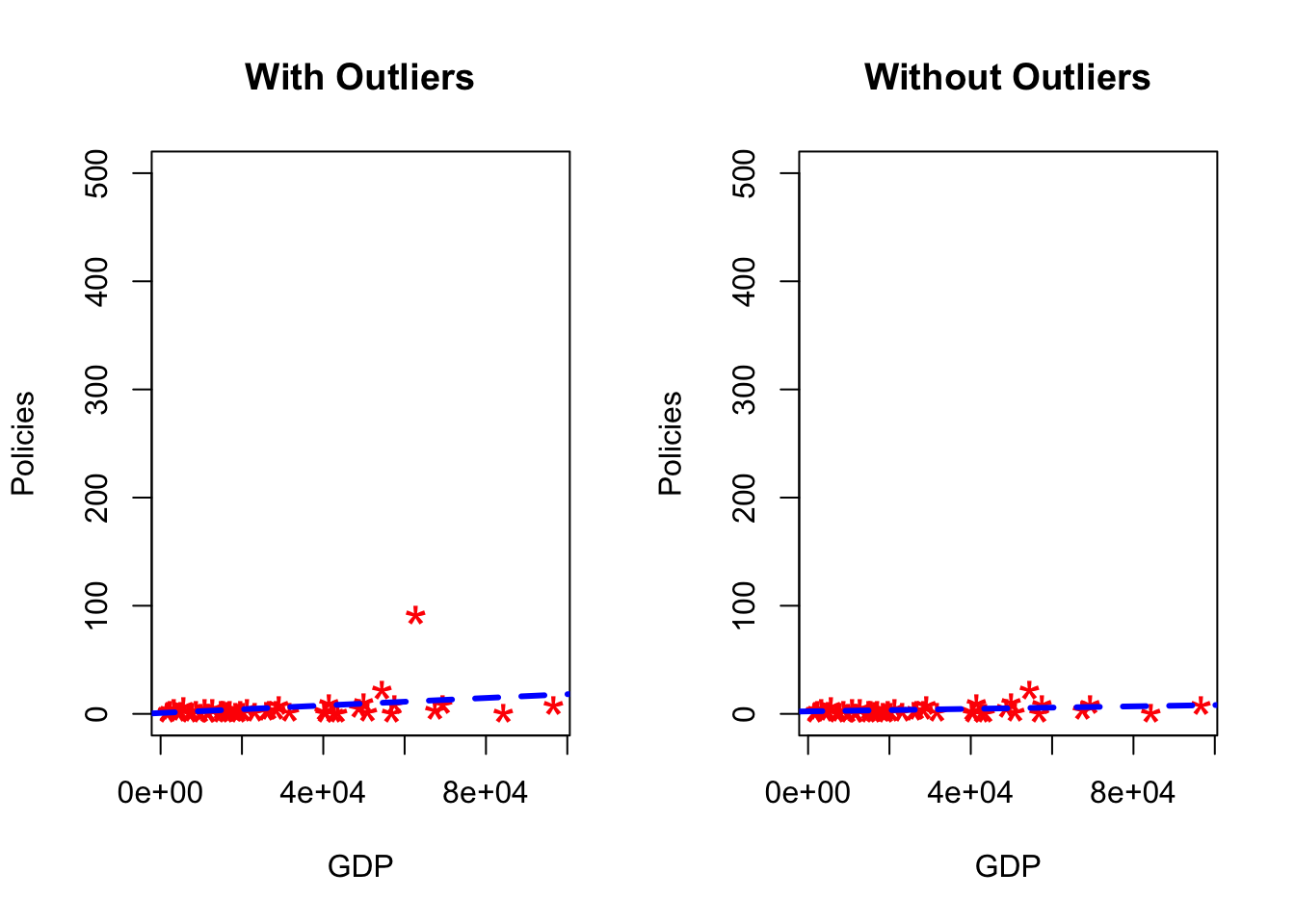
#Detect Outliers

par(mfrow=c(1, 1))
outlier_values <- boxplot.stats(dataAgg$numBusinessRestrictions)  # outlier values.
boxplot(dataAgg$numBusinessRestrictions, main="Outliers", boxwex=0.1)
mtext(paste("Outliers: ", paste(outlier_values, collapse=", ")), cex=0.6)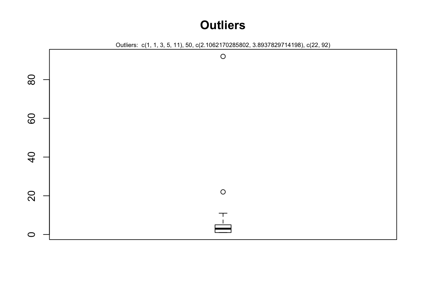
#Bivariate approach

# For categorical variable
boxplot(numBusinessRestrictions ~ date_announced, data=businessRestrictAgg,main="Ozone reading across months")  # clear pattern is noticeable.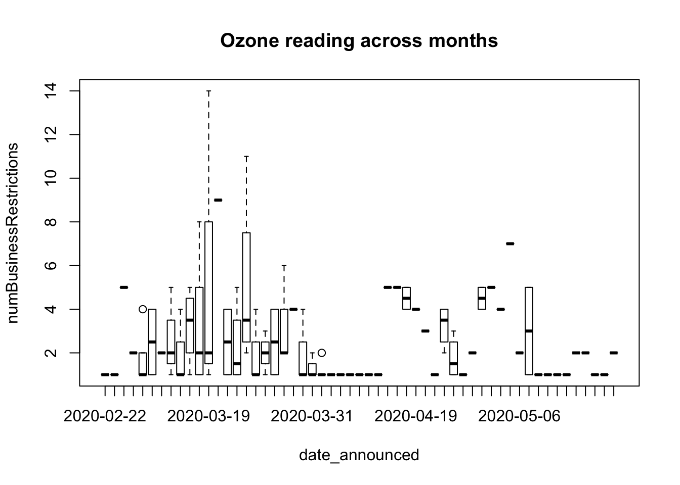
#Multivariate Model Approach
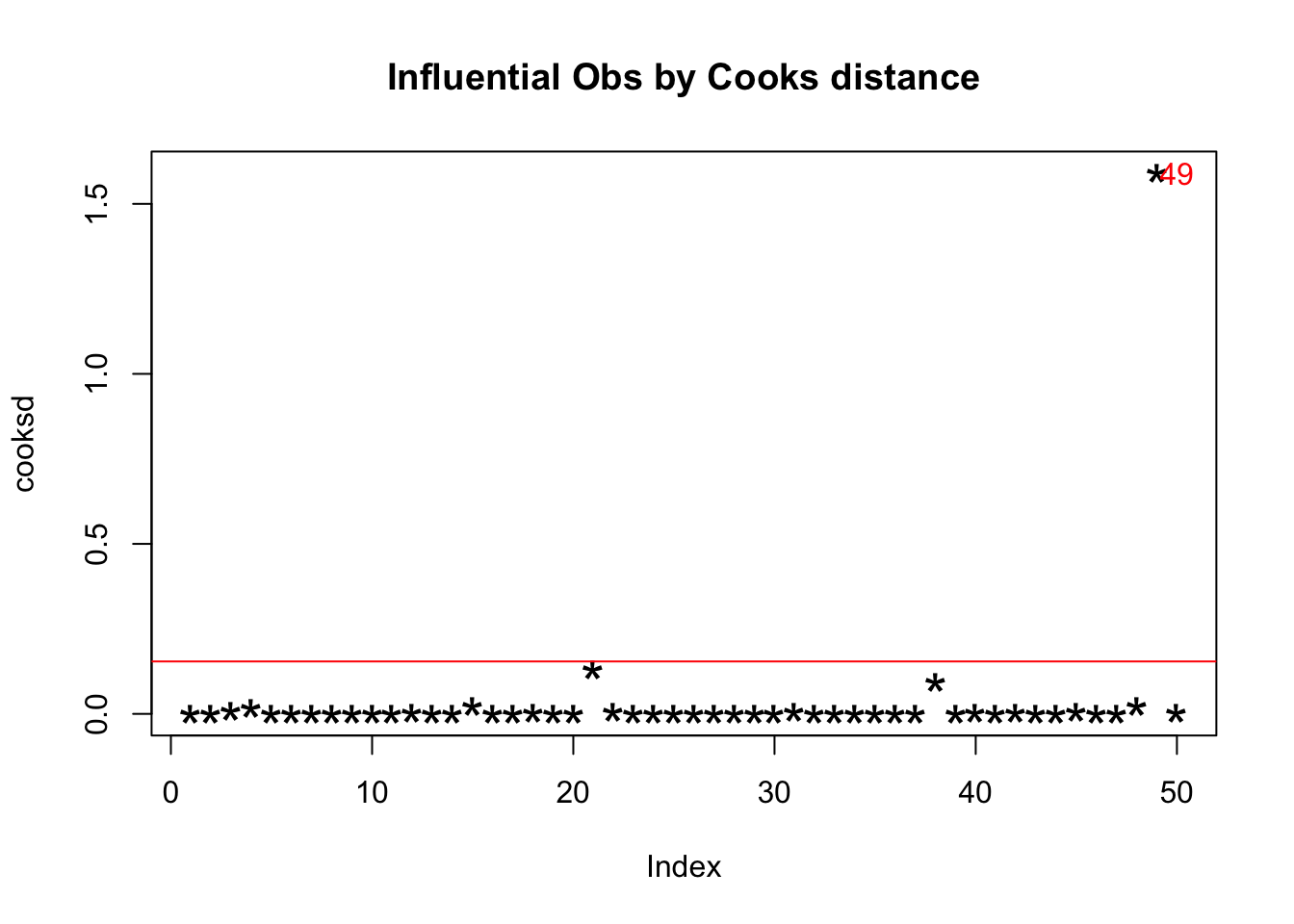
##Cooks distance
mod <- lm(numBusinessRestrictions ~ gdpPPP, data=dataAgg)
cooksd <- cooks.distance(mod)
plot(cooksd, pch="*", cex=2, main="Influential Obs by Cooks distance") # plot cook's distance
abline(h = 4*mean(cooksd, na.rm=T), col="red") # add cutoff line
text(x=1:length(cooksd)+1, y=cooksd, labels=ifelse(cooksd>4*mean(cooksd, na.rm=T),names(cooksd),""), col="red") # add labels