Download the script here. There are no exercises so this script contains all necessary code already.

Download the data here (same data as on the DataViz Eurostat page)

1 Tl;dr

This is how standard OLS regressions are done:

ols_object <- lm(regressand ~ regressor1 + regressor2 + regressor3,
                 data = data.frame)

This is how a (two-ways FE) panel regression is done

library(plm)
panel_object <-
   plm(
      regressand ~ regressor1 + regressor2 + regressor3,
      index = c("unit", "time"),
      model = "within",
      effect = "twoways",
      # for two-ways fixed effect regressions
      data = data.frame
   )

This is how you can get a summary of your regression:

summary(ols_object, panel_object)

This is a nicer way for getting a summary and exporting (journal style)

library(stargazer)
stargazer(ols_object, panel_object,
          type = "html", # either html, latex, or text
          out = "output.html") # if a file should be produced

2 Introduction

2.1 Workflow

2.2 The `lm` Function

lm(formula,
   data,
   subset,
   na.action)

formula - Specification of our regression model

data - The dataset containing the variables of the regression

subset - An option to subset the data

na.action - Option that specifies how to deal with missing values

2.3 The `formula` Argument

We can write our models using the following syntax:

model <- formula(regressand ~ regressors)

Where regressand is just our dependent variable / response usually denoted by $y$ and model is our formula of independent variables / regressors, e.g.:

kicker_success_formula <- formula(kicker_success ~ experience + training + luck)

We can construct formulas with the following syntax:

Adding variables with +

formula(y ~ a + b)

Interactions with :

formula(y ~ a + b + a:b)

Crossing: a * b is equivalent to a + b + a:b

formula(y ~ a + b + a:b) # and
formula(y ~ a * b) # are equivalent

Transformations with I()

formula(y ~ a + I(a ^ 2)) # quadratic term must be in I() to evaluate correctly
formula(y ~ log(a)) # log can stay by itself

Include all variables in your data with .

formula(y ~ .) # is equivalent to
formula(y ~ a + b + ... + z) # for a dataset with variables from a to z

2.4 The `subset` Argument

Sometimes, we want to run our model on a subset of our data (without changing the data themselves)
We can specify subsets of certain variables as follows:

lm(formula,
   data,
   subset = age < 30)

Connect multiple subset arguments with logical operators:

lm(formula,
   data,
   subset = age < 30 & height > 180)

Note that although this works, a best practice is to subset your data prior to the estimation. By keeping these steps distinct, your code will be much easier for someone else to understand.

2.5 The `na.action` Argument

If the data contains missing values, lm automatically deletes the whole observation.

Specify na.action = na.fail if you want an error when the data contains missing values

Again, it is a best practice to look for missing values in your data prior to the estimation to keep your code transparent.

You can use the missmap function from the Amelia package to get a nice visualisation of missing values in your data

2.6 Example Call of `lm` with Eurostat Data

eur_data <- read.csv2("data/eurostat_data.csv")

m1 <-
   formula(unemp_workagepop_t ~ gdp_gr + inv_per_empl + immigration_t,
           subset = year == 2014)
model <- lm(formula = m1,
            data = eur_data)

2.7 Output of `lm`

The lm function returns a list. Relevant components of this list are:

call - the function call that generated the output
coefficients the OLS coefficients
residuals
fitted.values The estimates for our dependent variable (unemployment)
model The model matrix used for estimation

The full list of outputs can be looked up via

?lm()
str(model) where model is our saved output from lm
the $ operator and tab, e.g. model$...

Lets look up our coefficients $\beta$, fitted values $\hat{y}$ and OLS residuals $\varepsilon$

model$coefficients

##   (Intercept)        gdp_gr  inv_per_empl immigration_t 
##  1.284087e+01 -1.636299e-01 -3.228256e-01 -2.266933e-06

model$fitted.values[1:7] # first 7 fitted values

##       14       15       16       17       18       19       20 
## 7.844069 9.367108 8.414682 8.144617 8.612589 8.671478 8.847128

model$residuals[1:7] # first 7 residuals

##        14        15        16        17        18        19        20 
## -3.644069 -3.967108 -3.514682 -3.544617 -3.712589 -3.271478 -3.147128

We can visualise the results very simply with hist or plot:

hist(model$residuals, breaks = 30)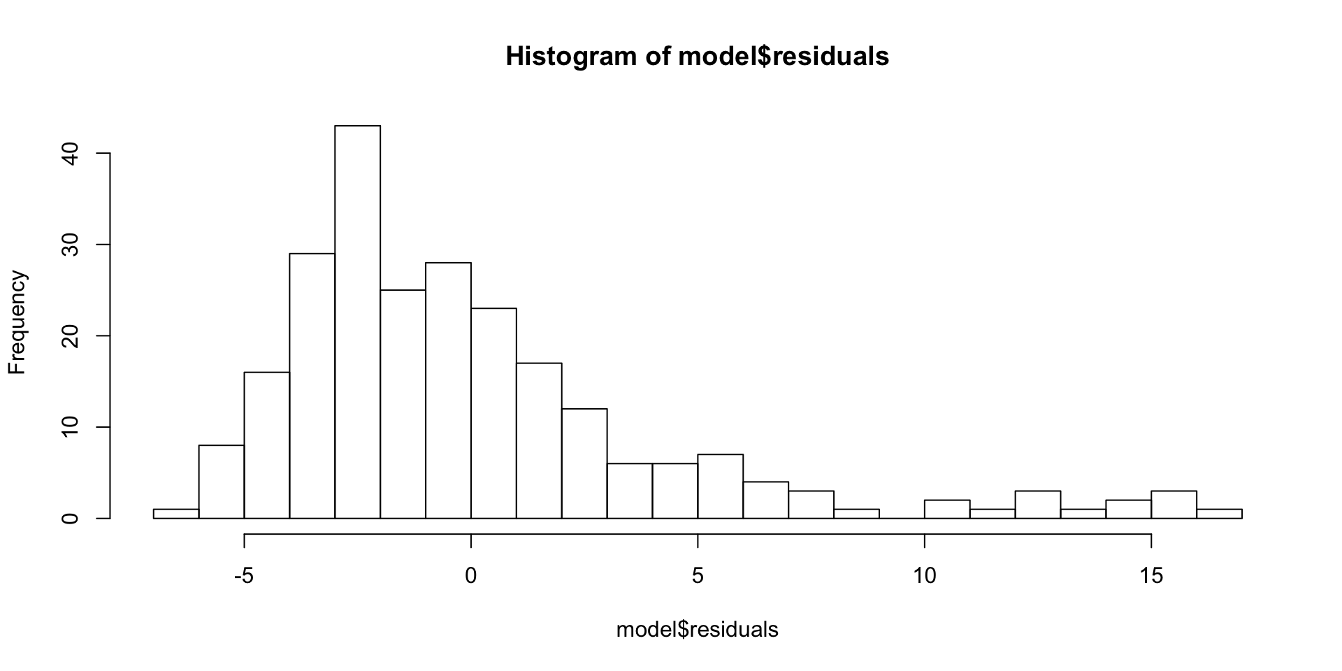

hist(model$fitted.values, breaks = 30)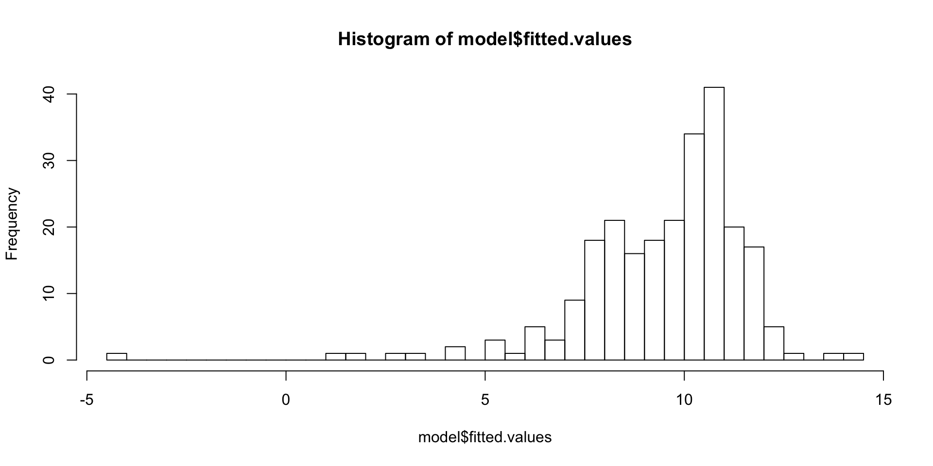

2.8 Output of `lm` with the `summary()` function

summary(model)

## 
## Call:
## lm(formula = m1, data = eur_data)
## 
## Residuals:
##    Min     1Q Median     3Q    Max 
## -6.446 -2.790 -1.099  1.529 16.458 
## 
## Coefficients:
##                 Estimate Std. Error t value Pr(>|t|)    
## (Intercept)    1.284e+01  5.628e-01  22.815  < 2e-16 ***
## gdp_gr        -1.636e-01  7.869e-02  -2.080   0.0386 *  
## inv_per_empl  -3.228e-01  5.039e-02  -6.406 7.91e-10 ***
## immigration_t -2.267e-06  1.438e-06  -1.576   0.1164    
## ---
## Signif. codes:  0 '***' 0.001 '**' 0.01 '*' 0.05 '.' 0.1 ' ' 1
## 
## Residual standard error: 4.386 on 238 degrees of freedom
##   (671 observations deleted due to missingness)
## Multiple R-squared:  0.1887, Adjusted R-squared:  0.1785 
## F-statistic: 18.46 on 3 and 238 DF,  p-value: 8.453e-11

2.9 Display and Export Tables with `stargazer()`

stargazer::stargazer(model, type = "text")

## 
## ===============================================
##                         Dependent variable:    
##                     ---------------------------
##                         unemp_workagepop_t     
## -----------------------------------------------
## gdp_gr                       -0.164**          
##                               (0.079)          
##                                                
## inv_per_empl                 -0.323***         
##                               (0.050)          
##                                                
## immigration_t                -0.00000          
##                              (0.00000)         
##                                                
## Constant                     12.841***         
##                               (0.563)          
##                                                
## -----------------------------------------------
## Observations                    242            
## R2                             0.189           
## Adjusted R2                    0.179           
## Residual Std. Error      4.386 (df = 238)      
## F Statistic           18.457*** (df = 3; 238)  
## ===============================================
## Note:               *p<0.1; **p<0.05; ***p<0.01

Jake Russ has the ultimate overview over all stargazer() functions (there are many!!).

2.9.1 Export Stargazer Output to File

stargazer::stargazer(model,
                     type = "html",
                     out = "model.html")

2.10 Compare different Models

model2 <- lm(unemp_workagepop_t ~ gdp_gr,
             data = eur_data)

stargazer::stargazer(model, model2,
                     type = "html")


	Dependent variable:

	unemp_workagepop_t
	(1)	(2)

gdp_gr	-0.164^**	-0.343^***
	(0.079)	(0.065)

inv_per_empl	-0.323^***
	(0.050)

immigration_t	-0.00000
	(0.00000)

Constant	12.841^***	9.152^***
	(0.563)	(0.258)


Observations	242	360
R²	0.189	0.071
Adjusted R²	0.179	0.069
Residual Std. Error	4.386 (df = 238)	4.423 (df = 358)
F Statistic	18.457^*** (df = 3; 238)	27.447^*** (df = 1; 358)

Note:	p<0.1; p<0.05; p<0.01

Specify the folder and file were your table should be saved as "path/name.type"

Output as .html : Open the file in your web browser and copy it into Word
Output as .tex : Include in LaTeX

3 Panel Regression

Just a very quick glimpse into panel regressions with plm.

library(plm)
panel_object <- plm(
   unemp_workagepop_t ~ gdp_gr,
   data = eur_data,
   index = c("geo_code", "time"),
   model = "within",
   effect = "twoways"
) # for two-ways fixed effect regressions

For further information on panel regressions, I recommend

the slides by Oscar Torres-Reyna
the Chapter 13 from the Econometrics with R book

Regression Analysis

1 Tl;dr

2 Introduction

2.1 Workflow

2.2 The lm Function

2.3 The formula Argument

2.4 The subset Argument

2.5 The na.action Argument

2.6 Example Call of lm with Eurostat Data

2.7 Output of lm

2.8 Output of lm with the summary() function

2.9 Display and Export Tables with stargazer()